Microsoft Excel formulas and features that you need to know
Microsoft Excel is ubiquitous, but it's far more than a simple spreadsheet app — a huge array of powerful features lay within its cells.

There are thousands of Excel tools at your disposal, so where should you start? Let's take a look at some of the basic formulas and advanced features of Microsoft Excel.
- SUM, COUNT and AVERAGE
- Adding IF
- Proper, UPPER and lower
- Search with VLOOKUP
- CONCATENATE
- Creating 3D Maps
- Freezing panes in Excel
- Using Pivot Tables
- Generating a Waterfall Chart
- Conditional Formatting
Basic Excel formulas
Before you attempt to hit the ground running, it's advisable to have a look at some of the basics to get you started.
The order and layout of a function and its arguments are known as the syntax. With Microsoft Excel, functions are built-in formulas which initiate the requested action on the information found in your worksheet. Formulas in Excel start with an equal sign (=), then continues with either a function name (SUM, COUNT, IF) or math operators and numbers. If we were to dissect this formula:
=COUNTIF(A1:E1, "Forecast")
We can break a formula down into the following parts:
- =COUNTIF — This is known as the function of the formula. COUNTIF allows you to count cells if they meet a criterion.
- A1:E1 — This is the range of cells that you want to count.
- "Forecast" — This is the parameter that we give when counting. In this case, we want to only want to count the cells that contain the word Forecast.
When selecting a single cell in a worksheet, you can either use your mouse to click on the cell or use your arrow keys to navigate to it. To select specific cells, select the first cell and then hold down CTRL. Then select the other cells in question.
SUM, COUNT and AVERAGE
One of the most frequent uses of Excel is capturing numerical data. Whether it's financial, quantity tracking or grade/score records, you can use Excel to easily manage them, saving you time.
All the latest news, reviews, and guides for Windows and Xbox diehards.
- SUM: Sum can be used to add numbers found in any cell, most commonly in a row or column. If you want to add up the total for numbers found in A1 to A10, you would enter
=SUM(A1:A10)into another cell. - COUNT: Count attacks the numbers in a different way. Instead of adding the value of the numbers in cells, Count will count and report on the number of cells that have a numerical value. Rather than manually counting how many of the one hundred cells in column B have numbers, you would type
=COUNT(B1:100)into another cell. - AVERAGE: The average option takes the average of the numerical values found within your selected range of cells. To take an average of the first 10 cells in column C, type
=AVERAGE(C1:C10)into another cell.
Adding IF
A small, two letter word can provide a lot of functionality to your data. If you were to use
=SUMIF(A1:A10,">10,000"), you have now chosen to find the sum of the numbers in the same cells, but only taking into account values that are greater than 10,000.
Proper, UPPER and lower
While functions such as proper, upper and lower aren't going to solve mathematical problems, they do ensure that the text is displayed correctly.
- PROPER: Proper will turn a string of text to the proper case by capitalizing the first letter in each word.
=PROPER(A1)will change john smith to John Smith. - UPPER: By using upper in a formula, such as
=UPPER(A1), you would change John Smith to JOHN SMITH. - LOWER: The Lower formula will change all alphabetical characters in targeted cells to lower case.
=LOWER(A1)would change John Smith to john smith.
VLOOKUP
VLOOKUP helps the user to search for specific data from a table and place it a new table. Let's say you have 10 items in a list with the item names in the first column and their price in the second column. You would want to type out the following in a nearby cell to find an item and its price:
=VLOOKUP("item name", A1:B10, 2, FALSE)VLOOKUP always searches the first column in a workbook. We've included column index number as a third argument since the prices are found in the second column.
CONCATENATE
This function can easily combine data from multiple cells into a single cell. It's a basic string function that helps to reduce the amount of data entry steps you have to take. If we were to use a phone number example, the formula could look like this:
=CONCATENATE(A1,B2,C3)This would then combine the area code, central office prefix and line number. Alternatively, you can also enter in
=A1&B1&C1to get the same result.
Advanced features of Excel
Those are some of the basic functions that an Excel user should know to be more efficient with their worksheets. Entering in data is one thing while manipulating the data to get information. Let's take a look at some even more useful features of Excel.
Creating 3D Maps
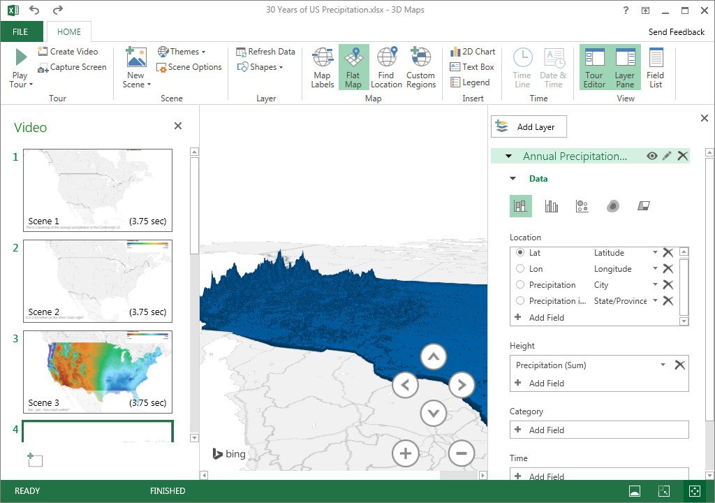
Even with the most organized database, some information and insight are lost if not visually engaging for the reader. With 3D Maps, you can generate a three-dimensional presentation of your data that can have a much larger impact on the data than numbers alone. Imagine being able to visually see changes to data over time and by geographical location.
Before you can begin using 3D Maps, you should make sure that your data contains some sort of geographic information within your tables. The data could contain details as complex as longitudes and latitudes or as simple as a zip code or postal code.
To create a 3D Map
- Open a workbook that contains a table of geographical details.
- Click Insert from the top ribbon.
- Click 3D Map under Tours.
- Click on the tour image, in the Launch 3D Maps popup, to begin editing Click on the tour image to begin editing.The information in your workbook Is geocoded, courtesy of Bing. 3D Maps will then open with your data presented in the areas listed in your workbook.
- Drag the fields from the Field list to the Layer pane as needed. The Field List box, next to the Layer pane on the right.
You can use any presented drop-down arrow in the fields to ensure the data is matched correctly to the right geodata. 3D Maps then works to plot the data on the globe in the areas recorded in your workbook. From this point, you can then create a presentation that can be recorded as a video, or interactive navigation for viewers to delve into. We'll take an in-depth look at navigating Power Map in a future article.
Freezing panes in Excel
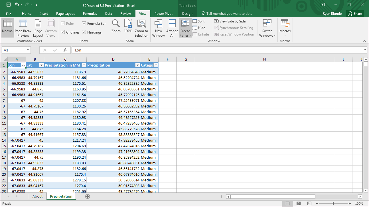
If you are working with a large database in Excel that requires navigating, it could be difficult to keep track of the which category belongs to which column or row. With the ability to freeze panes, Excel users can lock specific rows or columns in place so that they remain visible while you scroll up and down or side to side through cells.
To freeze rows or columns
- Click on View.
- Click on Free Panes under the Window section and choose from the following:
- Freeze Panes: Freezes the selected rows and columns in place. Depending on the placement of your cursor, you can use this option to lock more than one row or column. You can also lock rows and columns simultaneously.
- Freeze Top Row: Keeps the top row stationary, while the remaining panes can be scrolled through.
- Freeze First Column: This locks the first column only.
Using Pivot Tables
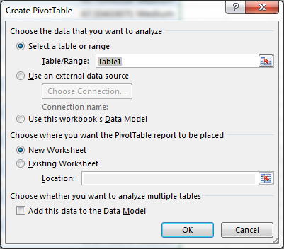
Pivot Tables are by far one of the most versatile ways to extract details from a large data set for further analysis. In a pivot table, data is sorted and summarized without necessarily having to input formulas to perform calculations.
To create a Pivot Table
- Click on Insert.
- Click on PivotTable.
- Verify your table/range values in the CreatePivot Table dialog box.
- Click on the PivotTable placement option that you need. Your options include:
- New Worksheet: This generates a new worksheet to begin to place your PivotTable.
- Existing Worksheet: This option asks where in the workbook you want to create the PivotTable. The table can be placed beside the existing data or even replace sections of it.
- Click OK to create a blank pivot table. A PivotTable Fields list will appear on the right side Excel.
- Click and drag your fields from Choose Fields to Add to Report to one of the four areas below:
- Report Filter: The Report filter aids to manage how large amounts of data are displayed while also helping to put the focus on data subsets.
- Column Labels: This section will decide the arrangement of the data found in the columns of the pivot table.
- Row Labels: As with Column Labels, this area determines how the data is shown in rows.
- Values: The Values section helps to decide which data will be displayed in the pivot table cells.
Recommended PivotTable is an optimal choice for those who are not familiar with PivotTables. Depending on the information in your workbook, Excel can create a PivotTable. This doesn't always work as you may have a high number of blank cells, duplicate values or too few numerical columns. In this case, you can still try to create a PivotTable yourself.
Waterfall charts
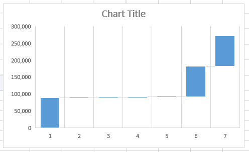
The Waterfall chart can capture the details of increase and decreases over time or any other type of change. The beginning and end columns normally represent the starting value and closing value, while the columns found in between will measure the changes, both positive and negative. This could be used to report on growth, revenue or even costs.
To create a Waterfall Chart
- Open the workbook and select the data to include in the chart.
- Click on Insert.
- Click on Waterfall or Stock Chart, under the Charts section.
- Select Waterfall.
- Position the resulting chart where you want on the workbook.
- Use Chart Layouts to change visible data and to add chart elements.
- Use Chart Styles to change colors and chart themes.
Conditional Formatting
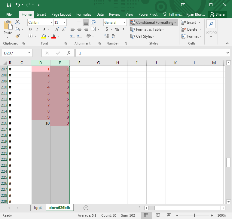
This Excel function helps the user to locate and visualize data within a worksheet. Through predefined rules, you can use conditional formatting to identify values using manyy criteria. Excel also provides the means to create rules of your own.
Let's use an example to learn basic conditional formatting. You're taking inventory and have two columns of tracking numbers; one from your system records and another that was manually entered. You can use conditional formatting the check the data.
To use Conditional Formatting
- Highlight the columns you want to use.
- Click on Home on the top bar.
- Click on Conditional Formatting under Styles.
- In the dropdown, choose Highlight Cells Rules.
- Select Duplicate Values.
- Choose to format cells that contain duplicate or unique values.
- Choose how to highlight cells with the chosen values.
This will then highlight any recorded tracking number that hasn't been scanned while also potentially highlighting tracking numbers scanned by not in the system.
Wrap Up
Again, this is but a few options that can be found in Microsoft Excel. It goes beyond creating a simple table of data. The numerical applications are complex in nature but will be simple to use over time. What does your work day with Excel look like? Do you excel at Excel? Let us know!

Ryan is a Former Contributor for Windows Central.
